This is an example for simulation of photon-deriven motor under MNDO calculation.
trajectory movie
Step 1: preperation of initial condition
Create a new directory:
Sampling initial conditions:
mpirun -np 8 ./kids -w -handler=sampling -d=winger_samp_50K -p param_wiger_sampling_50K.json
In the provided param_wiger_sampling_50K.json file, the parameters are specified as follows:
{
"model": "Interf_MNDO", // mndo interface
"mndoinp" : "S0.inp", // mndo input template
"exec_file": "mndo2020", // mndo executable file
"init_nuclinp" : "#hess", // initial sampling by Harmonic approximation
"hess_log": "zp_hess.out", // mndo log produced by frequency calculation (JOP=2 KPRINT=1)
"temperature": "50.0 K", // temperature for sampling
"classical_bath": false, // flag for wigner or classical distribution
"F": 2, // NO. of electronic states involved
"N": 90, // NO. of nulcear DOFs (3 x No. of atoms)
"M": 1000, // NO. of samples
"solver": "NAF-adapt", // Adaptive Integrator (not used in handler=sampling)
"dt": 0, // time step (not used in handler=sampling)
"occ": 0, // initial occupied state (numbering from 0)
}
In this configuration, S0.inp represents the minimum of the S0 state of the motor, while zp_hess.out contains the log file of the Hessian calculation for this structure (JOP=2 KPRINT=1). The contents of S0.inp resemble the following format:
JOP=-2 IOP=-6 IGEOM=1 IFORM=1 ICUTS=-1 ICUTG=-1 NSAV7=4 NSAV13=2 +
ISCF=9 IPLSCF=9 DPREC=1D-8 DSTEP=1D-5 IPRINT=1 +
NCIGRD=2 IEF=1 IPREC=100 +
IMULT=1 imomap=3 mapthr=95 +
KCI=5 IOUTCI=1 MPRINT=1 IUVCD=2 ICROSS=7 +
MOVO=0 ICI1=6 ICI2=3 NCIREF=3 MCIREF=0 LEVEXC=2 IROOT=3 KITSCF=250
This file is generated automatically
6 0.04380338793550 0 0.35077864691677 0 -0.10882721806895 0
6 1.27121168655916 0 -0.23979603265391 0 -0.10208501977209 0
6 2.84226287946701 0 -1.92652319997327 0 -0.09579012490127 0
6 2.65466322153261 0 0.34008820792743 0 0.04769625311877 0
6 -1.66527000184424 0 2.15037595470014 0 -0.63643785262607 0
6 -0.09037626881828 0 1.92025140395509 0 -0.29070923410677 0
6 0.20040960553294 0 2.48113248777928 0 1.08479762064004 0
8 2.85709734292449 0 1.62697083010599 0 -0.07327426390024 0
1 -2.13756286310946 0 2.97755695887732 0 -0.03354811552012 0
1 -1.79490161761576 0 2.33562930149058 0 -1.74596516994872 0
1 0.58016298640936 0 2.54792774220182 0 -0.97734602010758 0
1 1.17729539774138 0 2.25501127109489 0 1.43060350197030 0
1 -0.57814464898532 0 2.05183223242283 0 1.79183498981984 0
1 0.28460862204132 0 3.54051041950305 0 1.18549546962596 0
1 3.09488609181207 0 -3.07973921031701 0 -0.13332221609733 0
6 3.61236452215164 0 -0.75440449571611 0 0.04026746833597 0
1 4.61142564115244 0 -0.52382073151543 0 0.15976722920344 0
7 1.55843885154116 0 -1.63613870859904 0 -0.13877851677858 0
1 0.98250807404859 0 -2.40645279632863 0 -0.52658707768494 0
6 -3.34344788021834 0 -1.20692875542908 0 -0.02955012333173 0
6 -3.56856116615990 0 0.22243729700008 0 -0.20050925408584 0
6 -2.27946396293341 0 0.84912004673990 0 -0.33761888260090 0
6 -1.27176847168875 0 -0.18466608507948 0 -0.07635502292883 0
7 -1.91738252475071 0 -1.41686609558211 0 0.08211433345851 0
1 -4.50249697318154 0 0.71308015177610 0 -0.60361324565497 0
6 -1.28430653514342 0 -2.59490599037353 0 0.60434180765570 0
1 -0.96827978921506 0 -3.20081206711561 0 -0.22748342879066 0
1 -0.50639587335968 0 -2.34933980795280 0 1.36248208576779 0
1 -2.06980017157749 0 -3.13442523272339 0 1.37893965343842 0
1 -4.23683976135963 0 -1.89224882856376 0 0.09017577052527 0
0 0.000000000000000 0 0.00000000000000 0 0.00000000000000 0
1 2
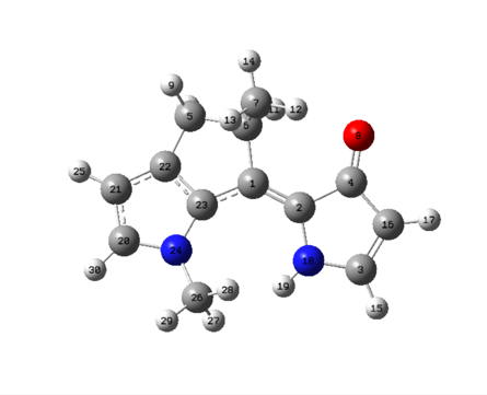
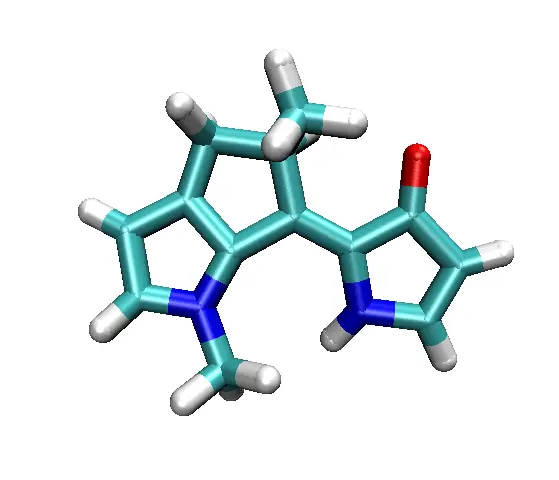
View of the molecular motor
List the contents of the winger_samp_50K/ directory:
ls winger_samp_50K/
## fort.13 fort.7 fort.91 molden.dat samp0.ds samp1.ds samp2.ds samp3.ds ...
All files named xxx.ds are generated by sampling using the Wigner distribution under Harmonic approximation. However, if classical_bath is set to true, the Boltzmann distribution is used instead. Prior to sampling, the initial structures undergo a filtering process based on frequency strength, $$ P_{if}^{(\alpha)} \propto f_{if}^{(\alpha)} / (E_i^{(\alpha)} - E_f^{(\alpha)})^2 $$ which is carried out by a Python script:
3
import numpy as np
import pandas as pd
import os
import sys
import re
def getfiles(path):
f_list_raw = os.listdir(path)
f_list = []
for i in f_list_raw:
if os.path.splitext(i)[1] == '.ds':
f_list += [i]
return f_list
if __name__ == '__main__':
path = sys.argv[1]
out_path = sys.argv[2]
from_size = int(sys.argv[3])
samp_size = int(sys.argv[4])
Nf=from_size
file_id = np.arange(Nf)
np.random.shuffle(file_id)
print(file_id)
frp = []
E1 = []
E2 = []
cnt = 0
for i in file_id:
print(cnt)
cnt+=1
frps = re.split("[ |\n]+", os.popen(
"cat %s | grep -A2 f_rp | tail -n 1"%(path + '/samp%d.ds'%i)
).read().strip() )
frp += [float(frps[1])]
Es = re.split("[ |\n]+", os.popen(
"cat %s | grep -A2 model.rep.E | tail -n 1"%(path + '/samp%d.ds'%i)
).read().strip() )
E1 += [float(Es[0])]
E2 += [float(Es[1])]
frp = np.array(frp)
E1 = np.array(E1)
E2 = np.array(E2)
v = frp / (E2-E1)**2
pd.DataFrame(np.vstack([file_id, frp, E1, E2, v]).T).to_csv(
out_path + '_dat.csv',
header=['id', 'frp', 'E1', 'E2', 'v'],
index=None
)
maxv = np.max(v)
samp_files = []
while len(samp_files) < samp_size:
print('#'*10)
r = np.random.random(size=(Nf))
idx = np.where(v > r*maxv)[0]
samp_files += list(file_id[idx])
samp_files = samp_files[:samp_size]
print(samp_files)
os.popen('mkdir %s'%out_path)
cnt = 0
for i in samp_files:
os.popen('cp %s %s'%(path + '/samp%d.ds'%i, out_path + '/init%d.ds'%cnt))
cnt += 1
To filter the initial structures based on frequency strength, utilize the Python script select_init.py. Execute the script with the following arguments: samp_dir (directory containing sampled structures), filter_dir (directory to store filtered structures), number_of_samp_ds (total number of sampled structures), and number_of_filter_ds (desired number of filtered structures).
For instance:
python3 select_init.py winger_samp_50K winger_filter_50K 1000 480
This command will filter 480 structures (saved in (.ds) format) from a total of 1000 sampled structures.
We also provide utils for analysis of initial sampling from (.ds) files, for example
# export A1=4; export A2=2; export A3=1; export A4=6
python stat_bond.py winger_filter_50K 480 bond_data A1 A2 # stat bonds
python stat_angle.py winger_filter_50K 480 angle_data A1 A2 A3 # stat angles
python stat_dihedral.py winger_filter_50K 480 dihedral_file A1 A2 A3 A4 # stat dihedral angles
And the reduced initial distribution is shown as:
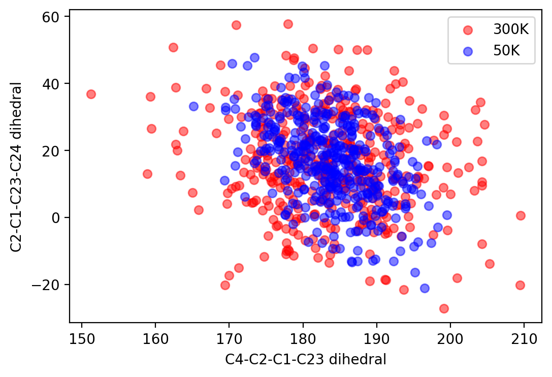
dihedral distribution
Step 2: run nonadiabatic simulation
An illustrative file represents a simulation conducted using NaF-TW:
// filename param_nad.json
{
"model": "Interf_MNDO",
"solver": "NAF-adapt",
"cmsh_flag": "CVSH",
"mndoinp" : "S0.inp",
"exec_file": "mndo2020",
"init_nuclinp" : "winger_samp_50K/init0.ds", # read initial condition from sampled (.ds) files
"F": 2,
"N": 90,
"occ": 1,
"dt": "0.5 fs",
"tend": "1000.0 fs",
"time_unit": "1.0 fs",
"msize": 1024, # max split of dynamics time step
"sstep": 4,
"M": 1,
"representation_flag" : "Adiabatic",
"gamma": 0.333333,
"hopping_type1": 1,
"hopping_type2": 2,
"reflect": false,
"use_cv" : true,
"sqc_init": 0,
"use_sqc" : true,
"only_adjust": false,
"conserve_scale": true,
"result": [
// the results you want to collect
]
}
One can perform the simulation by:
./
kids -w -handler=parallel -d init_from_0 -p param_nad.json
then each run will generate a res.dat file. And then can be treated with pandas.
statistic of breakdown trajectory
| Method | No. of traj. | breakdown |
| NaF-TW(old) | 398 (38,169) | 59 (43+15+1) |
| NaF-TW | 391 (17,56,71,126,185,241,204,331,363) | 52 (37+14+1) |
| NaF-TW2 | 397 (23,199,382) | 63 (47+16) |
| Ehrenfest | 399 (17) | 30 (24+6) |
| FSSH | 397 (184,191,230) | 61 (49+12) |
| NaF(1/3) | 391 (17,101,105,272,304,307,318,347,369) | 64 (50+13+1) |
| NaF(1/2) | 396 (107,237,333,359) | 47 (37+9+1) |
How to solve issue:
UNABLE TO ACHIEVE SCF CONVERGENCE … DIIS ERROR:Energy CONSERVATION ERROR: ...:ERROR: ENERGY SEPARATION FOR ACTIVE REDUNDANT PAIR:
after resampling of the breakdown trajectories
| Method | No. of traj. | breakdown |
| NaF-TW(old) | 398 (38,169) | 59 (43+15+1) |
| NaF-TW | 391 (17,56,71,126,185,241,204,331,363) | 52 (37+14+1) |
| NaF-TW2 | 397 (23,199,382) | 63 (47+16) |
| Ehrenfest | 399 (17) | 30 (24+6) |
| FSSH | 397 (184,191,230) | 61 (49+12) |
| NaF(1/3) | 391 (17,101,105,272,304,307,318,347,369) | 64 (50+13+1) |
| NaF(1/2) | 396 (107,237,333,359) | 47 (37+9+1) |
Step 3: analysis result
python get_dihedral.py MOD_0.333333_SQC1/motor_CVSH_12_rfalse_cvtrue_sqc0_i 400 dh_SQC1 4 2 1 6